A Basic Tutorial on Analyzing the Coronavirus Genome

@Michael_Okoko, as promised I’ve started working on the variant calling demonstration using SARS-CoV2 data.

I’m going to post the analysis in discrete steps, so that A) so that I can work on it a little bit at a time and B) allow questions before moving on to the next step.

Some housekeeping notes:

  • The reference genome I’m using is, I believe, the original genome sequenced from a patient in Wuhan. The sequence can be found here.
  • I’m using 100 samples for variant calling. All of them were downloaded from the Sequence Read Archive. The samples are all from the same BioProject - PRJNA656534. There were chosen entirely because this was the first result I found while searching.
  • Instructions and code for doing this analysis will be found here.

Caveat:
What I’m doing in this analysis is sort of silly and unnecessary for viral genomic data. As we saw in the paper you linked earlier, it’s perfectly possible to sequence and fully assemble the genomes of thousands of samples and use an alignment of the assemblies to call variants. But this approach is not currently practical or cost-effective for calling variants in most cellular organisms (particularly eukaryotes), so the general approach that I will walk through is the type of analysis that is typically done when we can’t assemble dozens/hundreds/thousands of genomes.

Okay, let’s first talk about the reference assembly of the SARS-CoV2 genome. Here is graphical view of the genome provided by NCBI:

The genome sequence is 29,903 RNA nucleotides in length, the majority of which consists of protein-coding genes. If you go to the NCBI link above, you can mouse over the various features and get a description of each of them.

I’m going to use the Integrative Genomics Viewer to visualize the results of this analysis. It’s free and easy to install on any operating system. You can find it here.

If we load the genome assembly into IGV, here is what we see:

There’s not much going on here yet, because the only thing we’ve loaded is the actual sequence, and we’ve viewing the full length of the sequence, so individual nucleotides are not visible. We can zoom in to take a closer look:

Now we’re looking at ~145 bp region in the middle of the genome. I believe this is part of the ORF1ab gene, but there is no information regarding gene annotations or other features – only the sequence itself.

Speaking of the sequence, here is what it looks like in the text file I downloaded (only the first 50 lines of the sequence are shown):

>NC_045512.2 Severe acute respiratory syndrome coronavirus 2 isolate Wuhan-Hu-1, complete genome
ATTAAAGGTTTATACCTTCCCAGGTAACAAACCAACCAACTTTCGATCTCTTGTAGATCTGTTCTCTAAACGAACTTTAA
AATCTGTGTGGCTGTCACTCGGCTGCATGCTTAGTGCACTCACGCAGTATAATTAATAACTAATTACTGTCGTTGACAGG
ACACGAGTAACTCGTCTATCTTCTGCAGGCTGCTTACGGTTTCGTCCGTGTTGCAGCCGATCATCAGCACATCTAGGTTT
CGTCCGGGTGTGACCGAAAGGTAAGATGGAGAGCCTTGTCCCTGGTTTCAACGAGAAAACACACGTCCAACTCAGTTTGC
CTGTTTTACAGGTTCGCGACGTGCTCGTACGTGGCTTTGGAGACTCCGTGGAGGAGGTCTTATCAGAGGCACGTCAACAT
CTTAAAGATGGCACTTGTGGCTTAGTAGAAGTTGAAAAAGGCGTTTTGCCTCAACTTGAACAGCCCTATGTGTTCATCAA
ACGTTCGGATGCTCGAACTGCACCTCATGGTCATGTTATGGTTGAGCTGGTAGCAGAACTCGAAGGCATTCAGTACGGTC
GTAGTGGTGAGACACTTGGTGTCCTTGTCCCTCATGTGGGCGAAATACCAGTGGCTTACCGCAAGGTTCTTCTTCGTAAG
AACGGTAATAAAGGAGCTGGTGGCCATAGTTACGGCGCCGATCTAAAGTCATTTGACTTAGGCGACGAGCTTGGCACTGA
TCCTTATGAAGATTTTCAAGAAAACTGGAACACTAAACATAGCAGTGGTGTTACCCGTGAACTCATGCGTGAGCTTAACG
GAGGGGCATACACTCGCTATGTCGATAACAACTTCTGTGGCCCTGATGGCTACCCTCTTGAGTGCATTAAAGACCTTCTA
GCACGTGCTGGTAAAGCTTCATGCACTTTGTCCGAACAACTGGACTTTATTGACACTAAGAGGGGTGTATACTGCTGCCG
TGAACATGAGCATGAAATTGCTTGGTACACGGAACGTTCTGAAAAGAGCTATGAATTGCAGACACCTTTTGAAATTAAAT
TGGCAAAGAAATTTGACACCTTCAATGGGGAATGTCCAAATTTTGTATTTCCCTTAAATTCCATAATCAAGACTATTCAA
CCAAGGGTTGAAAAGAAAAAGCTTGATGGCTTTATGGGTAGAATTCGATCTGTCTATCCAGTTGCGTCACCAAATGAATG
CAACCAAATGTGCCTTTCAACTCTCATGAAGTGTGATCATTGTGGTGAAACTTCATGGCAGACGGGCGATTTTGTTAAAG
CCACTTGCGAATTTTGTGGCACTGAGAATTTGACTAAAGAAGGTGCCACTACTTGTGGTTACTTACCCCAAAATGCTGTT
GTTAAAATTTATTGTCCAGCATGTCACAATTCAGAAGTAGGACCTGAGCATAGTCTTGCCGAATACCATAATGAATCTGG
CTTGAAAACCATTCTTCGTAAGGGTGGTCGCACTATTGCCTTTGGAGGCTGTGTGTTCTCTTATGTTGGTTGCCATAACA
AGTGTGCCTATTGGGTTCCACGTGCTAGCGCTAACATAGGTTGTAACCATACAGGTGTTGTTGGAGAAGGTTCCGAAGGT
CTTAATGACAACCTTCTTGAAATACTCCAAAAAGAGAAAGTCAACATCAATATTGTTGGTGACTTTAAACTTAATGAAGA
GATCGCCATTATTTTGGCATCTTTTTCTGCTTCCACAAGTGCTTTTGTGGAAACTGTGAAAGGTTTGGATTATAAAGCAT
TCAAACAAATTGTTGAATCCTGTGGTAATTTTAAAGTTACAAAAGGAAAAGCTAAAAAAGGTGCCTGGAATATTGGTGAA
CAGAAATCAATACTGAGTCCTCTTTATGCATTTGCATCAGAGGCTGCTCGTGTTGTACGATCAATTTTCTCCCGCACTCT
TGAAACTGCTCAAAATTCTGTGCGTGTTTTACAGAAGGCCGCTATAACAATACTAGATGGAATTTCACAGTATTCACTGA
GACTCATTGATGCTATGATGTTCACATCTGATTTGGCTACTAACAATCTAGTTGTAATGGCCTACATTACAGGTGGTGTT
GTTCAGTTGACTTCGCAGTGGCTAACTAACATCTTTGGCACTGTTTATGAAAAACTCAAACCCGTCCTTGATTGGCTTGA
AGAGAAGTTTAAGGAAGGTGTAGAGTTTCTTAGAGACGGTTGGGAAATTGTTAAATTTATCTCAACCTGTGCTTGTGAAA
TTGTCGGTGGACAAATTGTCACCTGTGCAAAGGAAATTAAGGAGAGTGTTCAGACATTCTTTAAGCTTGTAAATAAATTT

(Note: I have no idea why parts of the sequence are highlighted in green)

This is an incredibly common file format called the “fasta” format, which was created, I believe, by the developers of the FASTA sequence alignment software. The software has been largely supplanted by other methods, but the file format lives on.

In this format, the first line is a header or description and always starts with a “>”. The actual sequence starts on the next line and may be contained entirely in that line or wrap across multiple lines.

Note that the actual viral genome is made of RNA, but sequencing protocols typically reverse transcribe the RNA into complementary DNA sequence in which Uracil has been replaced with Thymine.

Next, lets take a look at the set of samples for which we’ll be calling variants.

I wrote a simple script that takes a list of 100 sample accession IDs and downloads the corresponding sequence data. Based on the BioProject metadata, I believe these sample are from the New Mexico Department of Health Scientific Laboratory and were collected in August of 2020.

Again, these samples were chosen entirely opportunistically and are likely not representative of anything in particular. Obviously, this is would not be a good study design if our goal was to say something useful about genetic variation in SARS-CoV2, but it should be okay okay for a simple tutorial.

Each sample is represented by two files. For example, accession SRR12638318 consists of these two files:

SRR12638318_1.fastq.gz  SRR12638318_2.fastq.gz

These data were produced via so-called “paired-end” sequencing. In this process, genomic DNA is sheared or fragmented into a range of sizes (typically a few hundred nucleotides, although this will vary depending on the particular protocol used). And then each end of the fragmented is sequenced, generally starting from the outside and moving inward. Here is an illustration from Illumina, the company who currently has the market cornered on this particular technology:

So for each DNA sequence fragment, we will have two “reads” – one (depicted as orange above) sequenced in the “forward” direction, and another (blue) sequence in the “reverse” direction. All of the forward reads go in one file, and all of the reverse reads go in another. Hence, two files per sample.

These data are in the “fastq” format, which is somewhat similar to “fasta” but a little more complicated. Here is what the data for a single read look like:

@SRR12638318.2 2 length=151
TGCCTGTACCAAGAAATTATGATTAGACTTACGAATGAGTAAATCTTCATAATTAGGGTTAAGCATGTCTTCAGAGGTGCAGATCACATGTCTTGGACAGTAAACTACGTCATCAAGCCAAAGACCGTTAAGTGTAGTTGTACCACAAGTT
+SRR12638318.2 2 length=151
11>>A1F3DFBFGFCBFG1GBBGHBGBGGHFHCACGBFHHGFGHHHHHFHAFGHHGHHGHHHHHHHHHHHHHHHHHGHHHHHGHHHHHHHHHHHHHHHHGHHHHHHHHGHHGHHHGGHGHHHHHHHGGGGGHHHHHHHHHHHHHHHHEHHH

The first line is the sequence identifier and starts with an “@”. Typically this line will provide information regarding the sequencing instrument, the position of the read in the flow cell, and whether the read is forward or reverse (among other things). But in this case the data have been downloaded from the SRA repository, and much of this information has been removed, leaving us with just the accession ID and the read length.

The second line contains the actual sequence for the read. Pretty straightforward.

The third line is mostly just a placeholder to separate the sequence line from the quality scores line. It always starts with a “+” and may optionally be followed by other information (a repeater of the identifier line in this case).

The fourth and final line consists of quality scores for each nucleotide in ASCII format. Basically, the sequencing machine attempts to estimate the probability that the base was incorrectly called. In the above, an “H” represents a PHRED quality score of 39, which is a 0.00013 chance of an error. That’s a very good score, although there are various sources of error that are not accounted for in PHRED scores (see here for more info).

That’s the fastq format in a nutshell. For each sequence, there are 8 total lines spread across two files (forward and reverse). Because of this, the data add up very quickly, and the files can end up taking up a lot of space.

In this case, though, we don’t have too many reads per sample. As we’ll see later, it simply doesn’t take all that much sequencing to thoroughly cover a 30,000 nucleotide genome!

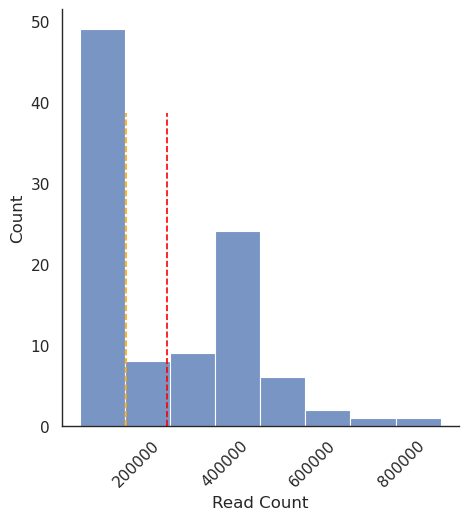
Here are the mean and median read counts:

Average reads per sample:       271432.66
Median reads per sample:        176628.0

And here is a histogram of the read count data, with mean and median highlighted by red and orange dashed vertical lines:

Now let’s look at the length of the reads:

Average read length:    117.49
Median read length:     136.0

image

I believe each forward and reverse read were originally ~150 base pairs in length (that’s the most common read length typically used in paired-end sequencing these days), but it appears that these reads have gone through some quality control that has altered the length distribution. Typically, the PHRED quality of the read decreases as the length of the sequenced molecule increases. Most QC tools will trim a read if the average length falls below some threshold. Therefore after QC, you get a large peak in the length distribution that is close to the original read length, followed by a tail of reads that have been trimmed to various lengths in order to remove low quality sequence data. That appears to be what happened here.

Okay, that was long and fairly boring, but hopefully the nature of the data we’re using is a little bit more clear. I’m going to leave it here for now and pick it back up tomorrow or in a couple days. The next step will be to align the reads to the reference genome.

In the meantime, feel free to let me know if there are any questions regarding things I didn’t cover or didn’t sufficiently clarify. I’m happy to correct any errors, so please point them out if you see any.

5 Likes

This is just amazing. Its only the first segment, but its very clear, detailed and straight to the point. Thanks for making out time to do this, I appreciate.

Do I have to download the script too? If yes, that means I have to download Python to run it? (I dabbled into programming a long time ago, but quit not long after. I am completely rusty in that area).

This is due to the relatively larger genome sizes of cellular organisms right?

I am not at home now, so I can’t fully follow along practically. When I set up the IGV software and successfully get to the same point as you, I will indicate. I will also share any queries with you. Thanks for your time again.

2 Likes

Thanks. I’m glad it’s helpful.

Do I have to download the script too? If yes, that means I have to download Python to run it? (I dabbled into programming a long time ago, but quit not long after. I am completely rusty in that area).

If you wanted to reproduce the analysis, yes you would need to install the miniconda package manager (which makes it easy to install software like python), download the code in that repository, and follow the additional steps to set up your environment with the correct software.

I should note that I’m doing this on a Linux server running the CentOS operating system. The analysis will probably work on a Mac. It will definitely not work on Windows.You might be able to get it to work by installing Unbuntu for Windows or something similar, but even then, I fear that trying to reproduce this may be an exercise in frustration if you are not on a native Linux/Mac machine. Most of the software used in modern genomics analysis simply isn’t designed to run on Windows. Sorry about that.

This is due to the relatively larger genome sizes of cellular organisms right?

Yes. Increasing both the size and repetitive content (edit: and ploidy!) of a genome drastically increases the monetary and computational cost associated with assembling the genome. I just finished assembling a new plant genome. It’s about 1 gigbase (1 billion bases) in size and consists roughly of 80% transposable elements. We sequenced it with with a newer technology that produces reads that are tens of thousands of bases in size but more error prone than the short reads.

This is currently the most practical way of assembling complex, repetitive genomes, which are nearly impossible to assemble with short reads. Even so, the assembly process took hundreds of thousands of CPU-hours to complete (around a month in actual human time), required using a machine with 100s of gigabytes of memory, and produced voluminous output of intermediate files that had to be stored somewhere at least temporarily.

Not all genomes are so computationally demanding to work with (humans aren’t quite as tough), and the technology–both the sequencing platforms and the software used to process the data–are improving all the time. But even so, it’s generally not practical to try to assemble dozens or hundreds of new eukaryotic genomes when you want to do a population analysis. Thus, we typically fall back to generating a single “reference” genome assembly from a single individual for the species in question, and then use read sequence alignment to find locations in the genome where individuals in the population differ from that reference sequence.

I am not at home now, so I can’t fully follow along practically. When I set up the IGV software and successfully get to the same point as you, I will indicate. I will also share any queries with you. Thanks for your time again.

Sounds good. I will place the final output file(s) in the git repository, which you could download even if you don’t want to do the full analysis.

1 Like

For a Windows 10 computer, I would strongly suggest installing Docker and then using one or more of the official Cyverse Vice images from DockerHub. Cyverse Vice provides a graphical environment that @Michael_Okoko might find easier to use. And running Docker images is certainly much, much easier than creating a new boot partition and installing Linux.

Caveat: I know nothing about genomics software; my suggestion is based on my long experience using Docker on Windows.

Best,
Chris

2 Likes

Just popping in to say that I haven’t forgotten about this. I’ve done the next step in the analysis, but I haven’t had a chance to write up a summary. I’ll do it soon(ish).

2 Likes

I managed to download the coronavirus reference sequence from NCBI and viewed it on IGV. Unfortunately, I won’t be able to do the full analysis due to the limitations you mentioned, but I can settle for the final output when you publish it. Thanks.

Is it possible to download the sequence data without scripts, that is, directly from the website?

It is possible, though it will be annoying to do so for a large number of samples. Here is what you do:

  1. Take one of the accession IDs from the list here. Let’s use “SRR13644077” for example.

  2. Optionally, you can search for it at NCBI’s Sequence Read Archive and get more information on the sample and the experiment it’s from.

  3. Proceed to the Run Browser and paste the accession ID into the search box and hit enter:

  4. Go to the “Reads” tab and click “Filtered Download”.

  5. Under “Download Format” select “fastq” and then click the Download link

  6. The file will be gzipped, so you will need to install a file archiving utility like Winzip or 7zip to extract the file. 7zip is free.

  7. Once the fastq file is extracted from the gzip archive, you can view in a text editor. The default program on windows, Notepad, is not very powerful but it will probably suffice. I recommend Notepad++ or Sublime if you’re going to work with text files often. Both are free.

I will try to write up the next steps in the analysis today or tomorrow.

2 Likes

Okay, so a brief recap:

We’ve downloaded and looked at the reference assembly for the SARS-CoV2 genome. And we’ve also downloaded ~100 sets of short read data from different samples.

The next step in the analysis is to try to figure out what part of the genome each of our reads originates from. To do this, we are going to “map” or “align” (for our purposes these words can be used interchangeably) each set of paired-end reads back to the assembly using a program called BWA-MEM. This process is similar in principle to a BLAST search, though the underlying algorithm is somewhat different, and it’s much, much faster. In the case of both programs, however, we take a subset of the query sequence, try to find a reliable match between it and the reference, and then attempt to extend the length of the match until we either A) run out of query sequence or B) the quality of the match falls below some threshold (due to mismatches or gaps).

I mapped each set of paired-end reads against the reference, running ~40 samples in parallel. The analysis took about 5 minutes to complete for all 100 samples. Notably, an equivalently scaled analysis of using average eukaryotic genome would take hours-to-days with the same amount of computational resources. There are several post-processing steps that I’m going to skip over, but the interested reader can take a look at the script for more detail.

The end result is a set of files in the BAM format, which is the binary equivalent of the “Sequence Alignment Map” format (SAM).

Here’s what an alignment in the SAM format looks like:

SRR12638349.34852       163     NC_045512.2     39      60      151M    =       78      190     ACTTTCGATCTCTTGTAGATCTGTTCTCTAAACGAACTTTAAAATCTGTGTGGCTGTCACTCGGCTGCATGCTTAGTGCACTCACGCAGTATAATTAATAACTAATTACTGTCGTTGACAGGACACGAGTAACTCGTCTATCTTCTGCAGG    BBBBBFBAFFFFGGGGGGGGGGHHHHHHHGHHHGGFGHHHHHFHHFHGEGFGDHHGHGGHHHGGGGCECHHGHHHGGFHHHHHHFHHGGEHGHFGHHHHHHGHHFHHHFHHGHGEFHHHHGGHHHHGGGGHHHHHGHGHHHHHHHHHHHHC

This is a single, tab-delimited line with 11 different columns, each providing a different piece of information. The format is explained in great detail, here. For our purposes, it’s enough to highlight the following:

  • column 1 shows the name of the read
  • column 2 lists a numerical “flag” that condenses a great deal of information regarding the nature of the read and the alignment into a single integer. A great website for decoding these flags is: SAM Format
  • column 3 shows the name of the sequence in the reference assembly (in this case there is only 1 sequence in the reference)
  • column 4 shows the position in the reference sequence where the alignment begins
  • column 5 shows a “Map Quality” score, which is the log-scaled probability that the mapper got the alignment position wrong. Higher numerical values represent more reliable alignments
  • column 6 shows a set of characters called a “CIGAR” string that represent a brief overview of the the alignment. Read more about this here: CIGAR string
  • columns 7 and 8 provide information regarding where (if anywhere) in the genome assembly the alignment for this read’s paired mate can be found
  • column 9 provides information that, roughly speaking, indicates the size of the genomic sequence fragment from which the paired end reads were generated
  • columns 10 and 11 show the full read sequence and base quality scores from the fastq file

For each read in the input fastq file(s), there will be an entry in the SAM file, even if no alignment was actually produced. Because of this, SAM files can balloon in size, very quickly. One way to save some space is the to convert the text-based SAM file to binary BAM format, at the cost of human readability. There are specialized programs (Samtools is the most popular) used to read BAM files and translate them back into human readable text and vice versa.

With those details out of the way, let’s actually get to the fun part and visualize the alignments…in the next post.

2 Likes

I’ve fired up IGV, loaded the reference assembly, and also loaded one of the alignment BAM files so that we can take a look.

(Note: please click on the images to expand them!)

Here is what the set of reads from sample SRR12638318 mapped against the reference looks like if we zoom out to the full extent possible:

Compared with our earlier look at IGV with just the assembly, there is an almost bewildering amount of information present here. So much so, that’s hard to see what’s going on.

A few points:

  • The reference sequence is shown at the top (zoomed out too far to make out the actual sequence)
  • Below that, there are two “tracks”. The firs track shows the coverage across the genome assembly. This indicates the number of reads that overlap any given position in the reference. If we look closely, we can see that the coverage varies from 0 reads to 4707 reads (that’s really high!). The second track shows a visual summary of the alignments against the assembly. Before we examine the alignments, let’s take a closer look at the coverage:

Here, I’ve enlarged the size of the coverage track and cropped out most of the alignments. We can see that the coverage is highly variable across the genome, although in most places it’s very high (100s of reads overlapping the same position). Interestingly, there is a region ~ the 21 Kb point where coverage drops almost to zero. I don’t know what’s going on with that. It might be worth looking to see if that same region has low coverage in other samples.

In general, higher coverage is good for variant calling because we can more reliably infer what the genotype of the sample should be and weed out true variants from sequencing and alignment error. That said, regions with anomalously high coverage may represent duplications or repeats that are hard to map accurately. Variant calling in such regions may be dicey.

Now let’s look at the aligned reads in a bit more detail. I’m going to zoom in quite a bit so that we can see what’s going on more clearly:

We’re now looking at a region that spans ~600 bp in the reference (note that the parallel black vertical lines simply represent the center of the view). The scale is such that we can now make out individual reads. We can see their orientation relative to the reference based on the direction of the arrows at one end of the read. The reads are colored blue or red based on which (cDNA) strand the first mate in a read pair was inferred to be on.

Single base mismatches from the reference are indicated by vertical lines, with different colored lines indicating different nucleotides (e.g., red vertical lines indicate “T”). We can see several mismatches that don’t appear to be found on very many reads (at least in the current zoomed view). These are probably sequencing errors that don’t represent true variants. However, we can also see a couple of “T” mismatches that are actually found in many different reads. More than likely, these represent true mutations present in the sample.

Another point worth noting is that you can click on any read, and a box will pop with loads of useful metadata about both the read and the base that’s present where you clicked:

Above, we can see essentially all the information present in the BAM file represented in a compact, user-friendly graphical view. IMO, IGV is an astonishingly well engineered piece of (free!) software.

If we scroll to a different position in the assembly, we can see that not all reads are created equal:

There are a handful of reads present here with many mismatches that aren’t present in most of the other reads. These are probably reads that are either misaligned or full of sequencing errors that were not trimmed by whatever QC process took place before the file was uploaded to the SRA. If we click on one of these reads, we see the following (note highlighted text):

The majority of the read has been “soft-clipped”, meaning that the mapping software considers only part of the read (60 bp) to have actually aligned to the reference. The rest of it has too many mismatches and fell bellow the alignment threshold. These soft-clipped regions will not be good candidates for variants and will likely be ignored by our variant calling software.

There is a lot more we could do with the alignments in IGV, but this is hopefully enough to get started. It’s really a fun program to play around with. We’ll use it again later.

The next step will be to repeat what we’ve just done visually–trying to differentiate true mutations from errors–under a much more robust mathematical framework that can take into account all the different samples at the same time. Fun!

It will probably be a few days again before my next post. Please let me know if there are any questions in the meantime.

3 Likes

It must be really painful since you keep contrasting the runtime for both types of analyses :smile:

I wonder how long it would take to analyze DNA sequences in tumors or cancer cells with multiple chromosomal duplications?

Is it possible to share the alignment BAM file here? I would like to actually see what you are teaching.

A bam file is in a format that is not human readable. He uses a program to read it, and posted images generated from that program already.

2 Likes

As @swamidass notes, a BAM file is a binary file, not a human readable text file.

Unfortunately, the text-based SAM files are impractically large for sharing over discourse (I think). Here are the first fifteen lines of one of the SAM files:

@HD     VN:1.6  SO:coordinate
@SQ     SN:NC_045512.2  LN:29903
@RG     ID:SRR13644091  SM:SRR13644091  LB:lib1 PL:ILLUMINA
@PG     ID:bwa  PN:bwa  VN:0.7.17-r1188 CL:bwa mem -R @RG\tID:SRR13644091\tSM:SRR13644091\tLB:lib1\tPL:ILLUMINA -t 40 assembly/GCF_009858895.2_ASM985889v3_genomic.fna fastqs/SRR13644091_1.fastq.gz fastqs/SRR13644091_2.fastq.gz
@PG     ID:samtools     PN:samtools     PP:bwa  VN:1.11 CL:samtools view -bS -o bams/SRR13644091.bam
@PG     ID:samtools.1   PN:samtools     PP:samtools     VN:1.11 CL:samtools sort --threads 40 -o bams/SRR13644091.sorted.bam bams/SRR13644091.bam
@PG     ID:MarkDuplicates       VN:Version:2.24.2       CL:MarkDuplicates --INPUT bams/SRR13644091.sorted.bam --OUTPUT bams/SRR13644091.sorted.markdup.bam --METRICS_FILE stats/SRR13644091.metrics.txt --MAX_SEQUENCES_FOR_DISK_READ_ENDS_MAP 50000 --MAX_FILE_HANDLES_FOR_READ_ENDS_MAP 8000 --SORTING_COLLECTION_SIZE_RATIO 0.25 --TAG_DUPLICATE_SET_MEMBERS false --REMOVE_SEQUENCING_DUPLICATES false --TAGGING_POLICY DontTag --CLEAR_DT true --DUPLEX_UMI false --ADD_PG_TAG_TO_READS true --REMOVE_DUPLICATES false --ASSUME_SORTED false --DUPLICATE_SCORING_STRATEGY SUM_OF_BASE_QUALITIES --PROGRAM_RECORD_ID MarkDuplicates --PROGRAM_GROUP_NAME MarkDuplicates --READ_NAME_REGEX <optimized capture of last three ':' separated fields as numeric values> --OPTICAL_DUPLICATE_PIXEL_DISTANCE 100 --MAX_OPTICAL_DUPLICATE_SET_SIZE 300000 --VERBOSITY INFO --QUIET false --VALIDATION_STRINGENCY STRICT --COMPRESSION_LEVEL 5 --MAX_RECORDS_IN_RAM 500000 --CREATE_INDEX false --CREATE_MD5_FILE false --GA4GH_CLIENT_SECRETS client_secrets.json --help false --version false --showHidden false --USE_JDK_DEFLATER false --USE_JDK_INFLATER false PN:MarkDuplicates
SRR13644091.52997       2147    NC_045512.2     12      60      19H64M67H       =       21552   21626   ATACCTTCCCAGGTAACAAACCAACCAACTTTCGATCTCTTGTAGATCTGTTCTCTAAACGAAC        GGGHHHHHHHHHGGHHHHHHGGHHGGFGGHHHHGGHHHHHHHHHHHGHHHHHHHHHHHHHGGGG        SA:Z:NC_045512.2,21552,+,73S77M,60,0;   MC:Z:65H86M     MD:Z:64 PG:Z:MarkDuplicates     RG:Z:SRR13644091        NM:i:0  AS:i:64 XS:i:0
SRR13644091.52997       2195    NC_045512.2     12      60      11H64M76H       =       21552   21478   ATACCTTCCCAGGTAACAAACCAACCAACTTTCGATCTCTTGTAGATCTGTTCTCTAAACGAAC        HGFGFHHGHGHHFHHHGHHGGGHEGF4@GGHGHHHHHHGHHHHHGHHHHGHHHHHHGHGGHHHH        SA:Z:NC_045512.2,21552,-,65S86M,60,0;   MC:Z:73H77M     MD:Z:64 PG:Z:MarkDuplicates     RG:Z:SRR13644091        NM:i:0  AS:i:64 XS:i:0
SRR13644091.51450       99      NC_045512.2     38      60      135M    =       38      135     AACTTTCGATCTCTTGTAGATCTGTTCTCTAAACGAACTTTAAAATCTGTGTGGCTGTCACTCGGCTGCATGCTTAGTGCACTCACGCAGTATAATTAATAACTAATTACTGTCGTTGACAGGACACGAGTAACT ABABAFFAAFFFGGGGFGFGGGHGGHHHGHHHHHGGGGHHHHHHHHFFHHGGHGHHGHHHHHHGGGGEGHHHHHHFHFGFGBGHGGHHGFGHHHGHHFFHGHHHHHHHHHHHFHGGGHHHHHGHHHHGGGGHGHH MC:Z:135M       MD:Z:135       PG:Z:MarkDuplicates      RG:Z:SRR13644091        NM:i:0  AS:i:135        XS:i:0
SRR13644091.51450       147     NC_045512.2     38      60      135M    =       38      -135    AACTTTCGATCTCTTGTAGATCTGTTCTCTAAACGAACTTTAAAATCTGTGTGGCTGTCACTCGGCTGCATGCTTAGTGCACTCACGCAGTATAATTAATAACTAATTACTGTCGTTGACAGGACACGAGTAACT GFGGHGHGHHHHGHHHHHGHHHHHHGHGHHEHGGGHHHHFHHHHHHHGGHHAHGBHHGFFGGGHHGHFGHHHHHHHHHGHHGFGEGHHHHHFHHHFFGHFGDF5FD5FHFCGGFFFGGGGGGGABFAFFFBAABA MC:Z:135M       MD:Z:135       PG:Z:MarkDuplicates      RG:Z:SRR13644091        NM:i:0  AS:i:135        XS:i:0
SRR13644091.7158        163     NC_045512.2     39      60      56M     =       39      56      ACTTTCGATCTCTTGTAGATCTGTTCTCTAAACGAACTTTAAAATCTGTGTGGCTG        @BBBBFB?FFFFGGFGGGGGGGGGHGHHHGHFHGFCEHHHHCHGHHHGHHHAEHHG        MC:Z:56M        MD:Z:56 PG:Z:MarkDuplicates     RG:Z:SRR13644091        NM:i:0  AS:i:56 XS:i:0
SRR13644091.9535        163     NC_045512.2     39      60      151M    =       137     249     ACTTTCGATCTCTTGTAGATCTGTTCTCTAAACGAACTTTAAAATCTGTGTGGCTGTCACTCGGCTGCATGCTTAGTGCACTCACGCAGTATAATTAATAACTAATTACTGTCGTTGACAGGACACGAGTAACTCGTCTATCTTCTGCAGG CDDCCFCBFFFFGGGGGGGGGGGHHHHHHHHHHGGGGHHHHGHHHHHHHHGHGHHGHHHHHHGGGGGGHHHHHHHHHFHHHGHHHHHGGGHHHHHHHGHGHHHHHHGHHHHHGGFFHHHHHGHHHHGGGEHHHHHGHGHHHHHHGHHHHHHMC:Z:151M        MD:Z:151        PG:Z:MarkDuplicates     RG:Z:SRR13644091        NM:i:0  AS:i:151        XS:i:0
SRR13644091.29405       1123    NC_045512.2     39      60      97M     =       39      97      ACTTTCGATCTCTTGTAGATCTGTTCTCTAAACGAACTTTAAAATCTGTGTGGCTGTCACTCGGCTGCATGCTTAGTGCACTCACGCAGTATAATTA      BCCCCFCCFFFFGGGFGGGGGGHFHHHHHHHHHGGGGHHHHHHHHHHHHHHHGHHGHHHHHHGGGGGGHHHHHHHHHHHHHHHHHHHGGGHHHHHHH        MC:Z:97M        MD:Z:97 PG:Z:MarkDuplicates     RG:Z:SRR13644091        NM:i:0  AS:i:97 XS:i:0
SRR13644091.51713       2147    NC_045512.2     39      60      37M99H  =       27041   27107   ACTTTCGATCTCTTGTAGATCTGTTCTCTAAACGAAC   CCCCCFCCFFFFGGGGGGGGGGHHHHHHHHHHHGGGG   SA:Z:NC_045512.2,27041,+,31S105M,60,0;  MC:Z:31H105M    MD:Z:37 PG:Z:MarkDuplicates     RG:Z:SRR13644091        NM:i:0  AS:i:37 XS:i:0

The first seven lines (each starting with “@” contain metadata about the reference genome, the sample, and the analyses that were performed. The final 8 lines contain the alignments between the reads and the reference.

If you PM me your email address, I’ll send you an email with one of the SAM files.

It’s not too painful if you’ve got enough CPUs to throw at the problem, though I suppose I’ve learned to calibrate my expectations, so some analyses that run in “only” a few hours seem pretty quick to me.

I haven’t personally analyzed genomic data with chromosomal abnormalities, but it’s certainly something that people do.

I know. I set up IGV on my PC, that’s why I asked for the file so that I follow the tutorial hands-on.

1 Like

Looking at the installation instructions, it seems I must use a command line. Will it work on Windows 8 (my PC OS)?

It seems you have become desensitized to the pain :smile:

My current PC would buckle on the computing load for complex genomes or possibly even this SARS-CoV-2 variant analysis. She is an old head and in dire need of replacement. I suspect you don’t use a laptop for your regular type of analysis?

Yeah, but I suspect they would be more computationally intensive to analyze relative to normal human cells. I saw a scary karyogram of some tumor cells: some chromosomes had four copies, others three. Variant analysis of those cells should require more than the usual.